Analysing differential phase contrast data

Example of a paper doing this type of data processing: Strain Anisotropy and Magnetic Domains in Embedded Nanomagnets. The data and processing scripts used in this paper is available at Zenodo with the DOI 10.5281/zenodo.3466591.

Differential phase contrast analysis (DPC) is done using using the DPCSignal classes: DPCSignal2D, DPCSignal1D and DPCBaseSignal.

Here, a test dataset is used to show the methods used to process this type of data. For information on how to load your own data, see :ref:load_dpc_data.

>>> import pixstem.api as ps
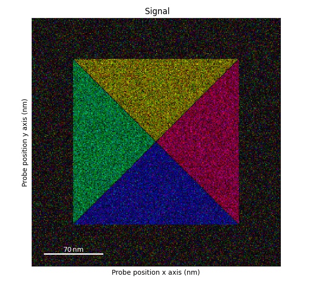
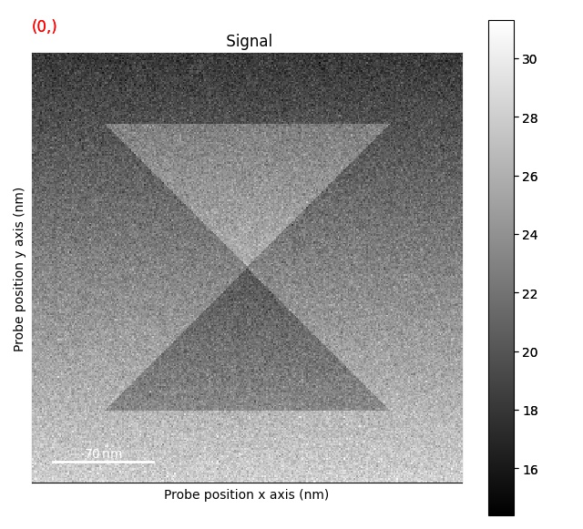
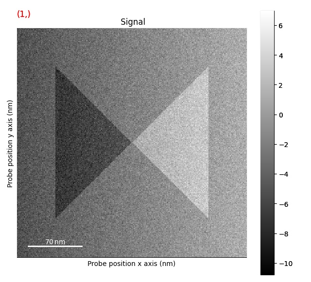
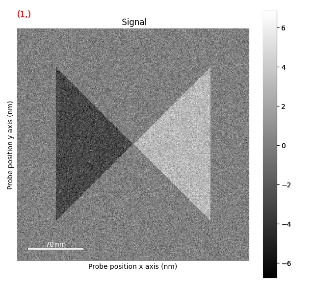
>>> s = ps.dummy_data.get_square_dpc_signal(add_ramp=True)
>>> s.plot()

Correcting d-scan

correct_ramp()

The first step is the remove the effects of the d-scan:

>>> s = s.correct_ramp()
>>> s.plot()

Note that this method only does a plane correction, using the corners of the signal. For many datasets, this will not work very well. Possibly tweaks is to change the corner size.

Plotting methods

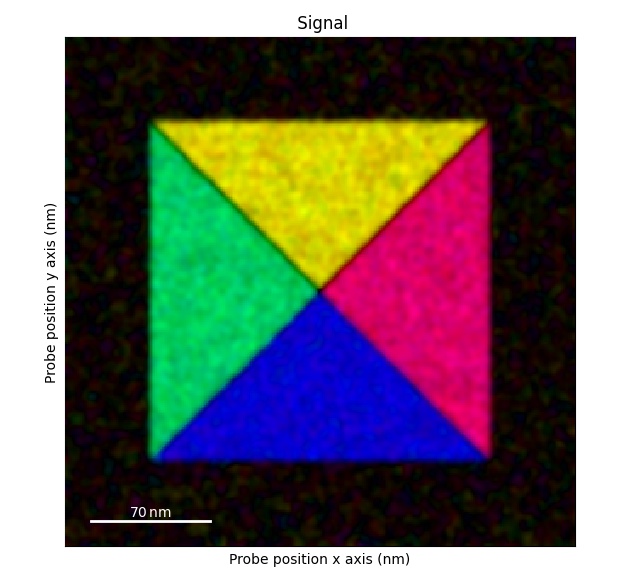
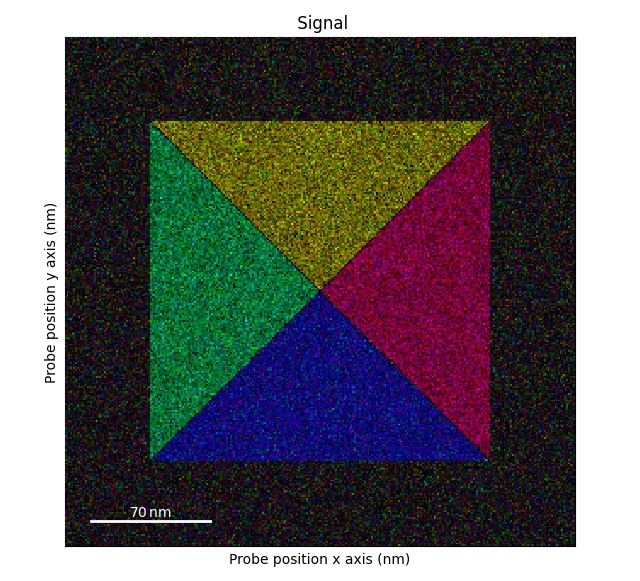
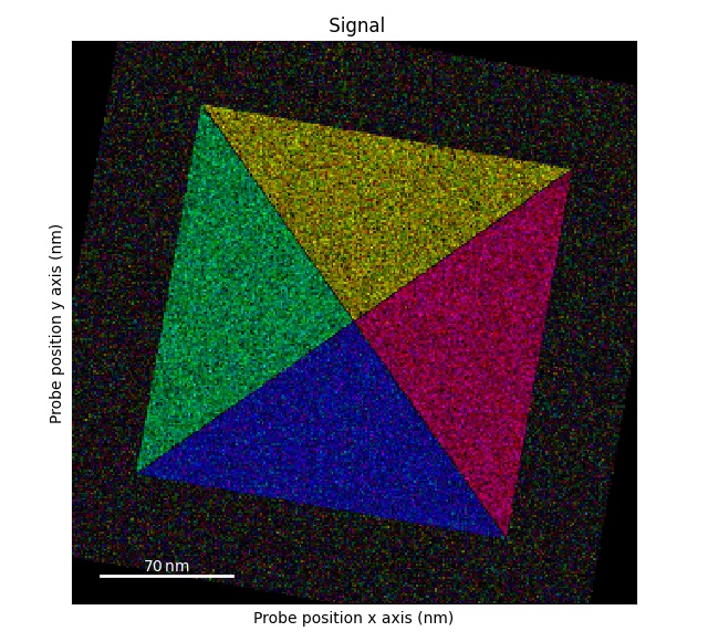
Plotting DPC color image using: get_color_signal()

>>> s_color = s.get_color_signal()
>>> s_color.plot()

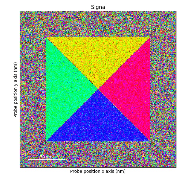
Plotting DPC phase image: get_phase_signal()

>>> s_phase = s.get_phase_signal()
>>> s_phase.plot()

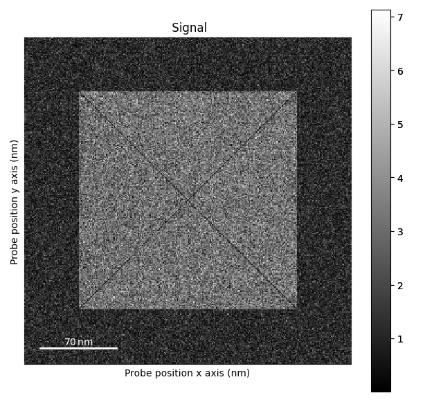
Plotting DPC magnitude image: get_magnitude_signal()

>>> s_magnitude = s.get_magnitude_signal()
>>> s_magnitude.plot()

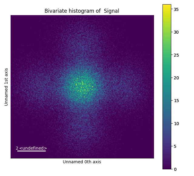
Plotting bivariate histogram: get_bivariate_histogram()

>>> s_hist = s.get_bivariate_histogram()
>>> s_hist.plot(cmap='viridis')

Plotting color image with more customizability: get_color_image_with_indicator()

>>> fig = s.get_color_image_with_indicator()
>>> fig.show()

Rotating the data

Rotating the probe axes: rotate_data(). Note, this will not rotate the beam shifts.

>>> s_rot_probe = s.rotate_data(10)
>>> s_rot_probe.get_color_signal().plot()

Rotating the beam shifts: rotate_beam_shifts().

>>> s_rot_shifts = s.rotate_beam_shifts(45)
>>> s_rot_shifts.get_color_signal().plot()

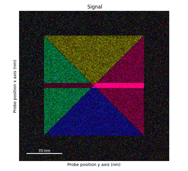
Rotating both the probe dimensions and beam shifts by 90 degrees: flip_axis_90_degrees(). Note: in this dataset there will not be any difference compared to the original dataset. So we slightly alter the dataset.

>>> s1 = s.deepcopy()
>>> s1.data[0, 50:250, 145:155] += 5
>>> s1.get_color_signal().plot()
>>> s_flip_rot = s1.flip_axis_90_degrees()
>>> s_flip_rot.get_color_signal().plot()

Blurring the data

The beam shifts can be blurred using gaussian_blur().

This is useful for suppressing the effects of variations in the crystal structure.

>>> s = ps.dummy_data.get_square_dpc_signal()
>>> s_blur = s.gaussian_blur()
>>> s.get_color_signal().plot()
>>> s_blur.get_color_signal().plot()