Using the pixelated STEM class

The PixelatedSTEM class extends HyperSpy’s Signal2D class, and makes heavy use of the lazy loading and map method to do lazy processing.

Visualizing the data

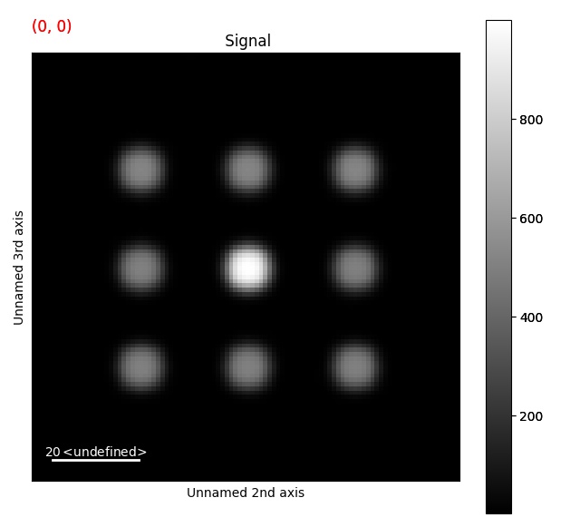
If you have a small dataset, s.plot can be used directly:

>>> import pixstem.api as ps
>>> s = ps.dummy_data.get_holz_simple_test_signal()
>>> s.plot()

If the dataset is very large and loaded lazily, there are some tricks which makes it easier to visualize the signal. Using s.plot() on a lazy signal makes the library calculate a navigation image, which can be time consuming. See HyperSpy’s big data documentation for more info. Some various ways of avoiding this issue:

>>> import pixstem.api as ps
>>> s = ps.dummy_data.get_holz_simple_test_signal(lazy=True)

Using the navigator slider:

>>> s.plot(navigator='slider') 

Using another signal as navigator, generated using virtual_annular_dark_field() or virtual_bright_field():

>>> s_adf = s.virtual_annular_dark_field(25, 25, 5, 20, show_progressbar=False)
>>> s.plot(navigator=s_adf)
>>> s_bf = s.virtual_bright_field(25, 25, 5, show_progressbar=False)
>>> s.plot(navigator=s_bf)

Center of mass

center_of_mass()

>>> s_com = s.center_of_mass(threshold=2, show_progressbar=False)
>>> s_com.plot()

Radial average

radial_average()

>>> s.axes_manager.signal_axes[0].offset = -25
>>> s.axes_manager.signal_axes[1].offset = -25
>>> s_r = s.radial_average(show_progressbar=False)
>>> s_r.plot()

Rotating the diffraction pattern

rotate_diffraction()

>>> s = ps.dummy_data.get_holz_simple_test_signal()
>>> s_rot = s.rotate_diffraction(30, show_progressbar=False)
>>> s_rot.plot()

Shifting the diffraction pattern

shift_diffraction()

>>> s = ps.dummy_data.get_disk_shift_simple_test_signal()
>>> s_com = s.center_of_mass(threshold=3., show_progressbar=False)
>>> s_com -= 25 # To shift the centre spot to (25, 25)
>>> s_shift = s.shift_diffraction(
...     shift_x=s_com.inav[0].data, shift_y=s_com.inav[1].data,
...     interpolation_order=3, show_progressbar=False)
>>> s_shift.plot()

Finding and removing bad pixels

find_dead_pixels() find_hot_pixels() correct_bad_pixels()

Removing dead pixels:

>>> s = ps.dummy_data.get_dead_pixel_signal()
>>> s_dead_pixels = s.find_dead_pixels(show_progressbar=False, lazy_result=True)
>>> s_corr = s.correct_bad_pixels(s_dead_pixels)

Removing hot pixels, or single-pixel cosmic rays:

>>> s = ps.dummy_data.get_hot_pixel_signal()
>>> s_hot_pixels = s.find_hot_pixels(show_progressbar=False, lazy_result=True)
>>> s_corr = s.correct_bad_pixels(s_hot_pixels)

Or both at the same time:

>>> s_corr = s.correct_bad_pixels(s_hot_pixels + s_dead_pixels)
>>> s_corr.compute(progressbar=False)  # To get a non-lazy signal

correct_bad_pixels() returns a lazy signal by default, to avoid large datasets using up excessive amount of memory.

Template matching with a disk or ring

template_match_disk()

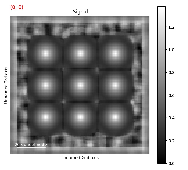
Doing template matching over the signal (diffraction) dimensions with a disk. Useful for preprocessing for finding the position of the diffraction disks in convergent beam electron diffraction data.

>>> s = ps.dummy_data.get_cbed_signal()
>>> s_template = s.template_match_disk(disk_r=5, lazy_result=False, show_progressbar=False)
>>> s_template.plot()

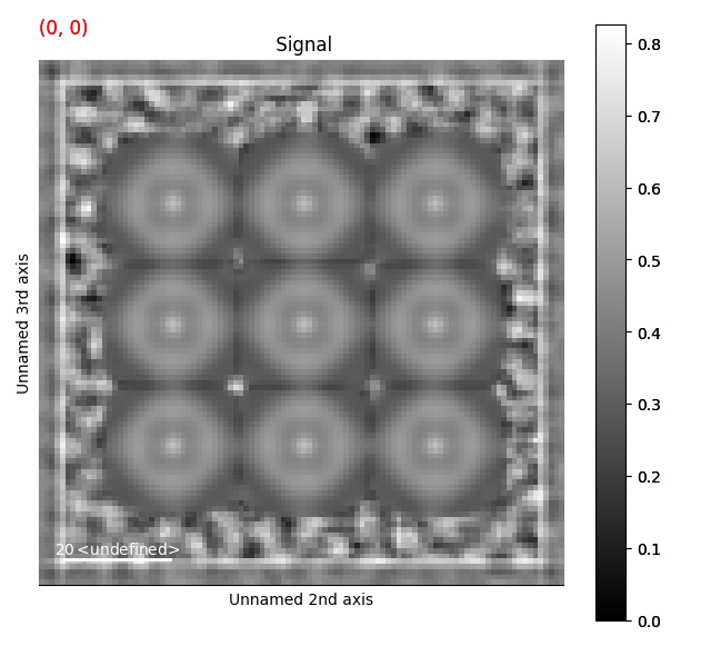
This can also be done using a ring template: template_match_ring()

>>> s = ps.dummy_data.get_cbed_signal()
>>> s_template = s.template_match_ring(r_inner=3, r_outer=5, lazy_result=False, show_progressbar=False)
>>> s_template.plot()

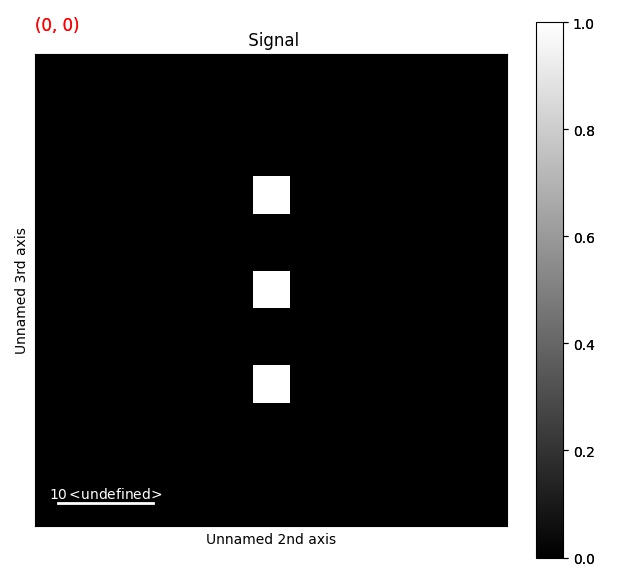
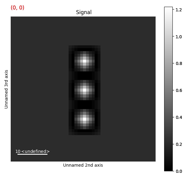
Template matching with any binary image

template_match_with_binary_image()

Any shape input image can be used for the template matching.

>>> import numpy as np
>>> data = np.zeros((2, 2, 50, 50))
>>> data[:, :, 23:27, 23:27] = 1
>>> data[:, :, 13:17, 23:27] = 1
>>> data[:, :, 33:37, 23:27] = 1
>>> s = ps.PixelatedSTEM(data)
>>> binary_image = np.zeros((8, 8))
>>> binary_image[2:-2, 2:-2] = 1
>>> s_template = s.template_match_with_binary_image(binary_image, show_progressbar=False, lazy_result=False)
>>> s_template.plot()

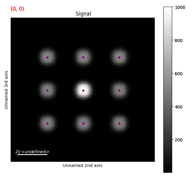
Peak finding

find_peaks()

For a more extensive example of using this functionality, see the nanobeam electron diffraction example.

Use scikit-image’s Difference of Gaussian (DoG) function to find features in the signal dimensions. For more information about the different parameters, see scikit’s documentation.

>>> s = ps.dummy_data.get_cbed_signal()
>>> peak_array = s.find_peaks(lazy_result=False, show_progressbar=False)
>>> peaks11 = peak_array[1, 1]

To visualize this, the peaks can be added to a signal as HyperSpy markers. For this, use add_peak_array_to_signal_as_markers().

>>> s.add_peak_array_as_markers(peak_array, color='purple', size=18)
>>> s.plot()

For some data types, especially convergent beam electron diffraction, using template matching can improve the peak finding:

>>> s = ps.dummy_data.get_cbed_signal()
>>> s_template = s.template_match_disk(disk_r=5, show_progressbar=False)
>>> peak_array = s_template.find_peaks(show_progressbar=False)
>>> peak_array_computed = peak_array.compute()

Note: this might add extra peaks at the edges of the images.