Analysing HOLZ datasets

In pixelated scanning transmission electron microscopy (STEM) datasets the higher order Laue zone (HOLZ) rings can be used to get information about the structure parallel to the electron beam. The radius of these rings are proportional to the square root of the size of the crystal’s unit cell size. This guide will show how to extract the size, intensity and width of HOLZ rings. These parameters can then be used to infer information about the crystal structure of a crystalline material.

Example of this type of data processing: Three-dimensional subnanoscale imaging of unit cell doubling due to octahedral tilting and cation modulation in strained perovskite thin films. The data and processing scripts used in this paper is available at Zenodo with the DOI 10.5281/zenodo.3476746, and an optimized Medipix3 dataset can be downloaded directly at: https://zenodo.org/record/3687144/files/m004_LSMO_LFO_STO_medipix_rechunked.hspy.

Loading dataset

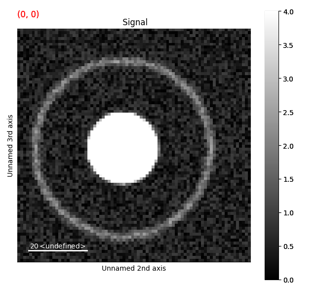
This example will use a test dataset, containing disk and a ring. The dataset is found in pixstem.dummy_data.get_holz_heterostructure_test_signal() The disk represents the STEM bright field disk, while the ring represents the HOLZ ring.

>>> import pixstem.api as ps
>>> s = ps.dummy_data.get_holz_heterostructure_test_signal()

Your own data can be loaded using pixstem.io_tools.load_ps_signal():

>>> import pixstem.api as ps
>>> s = ps.load_ps_signal(yourfilname)  

If you want to work with a real dataset, you can download the HOLZ dataset from Zenodo mentioned above. Note that this will download a 500 MB file.

>>> import urllib.request
>>> urllib.request.urlretrieve('https://zenodo.org/record/3687144/files/m004_LSMO_LFO_STO_medipix_rechunked.hspy', 'm004_LSMO_LFO_STO_medipix_rechunked.hspy')  
>>> import pixstem.api as ps
>>> s = ps.load_ps_signal('m004_LSMO_LFO_STO_medipix_rechunked.hspy', lazy=True)  

In some cases, the datasets might be too large to load into memory. For these datasets, lazy loading can be used. For more information on this, see Loading data.

Visualizing the data

The data is loaded as an PixelatedSTEM object, which extends HyperSpy’s Signal2D class. All functions which are present Signal2D is also in the PixelatedSTEM class.

>>> s
<PixelatedSTEM, title: , dimensions: (40, 40|80, 80)>

The (40, 40|80, 80) shows the dimensions of the dataset: 40 x 40 probe positions, and 80 x 80 detector pixels.

To visualize the dataset, we use:

>>> s.plot()

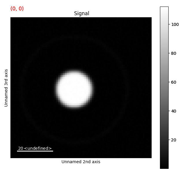
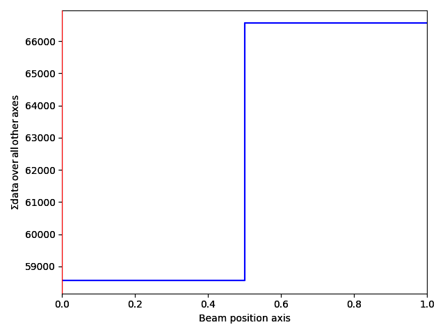
Drag the red box (lower right corner in the navigation plot) change the probe position. See the HyperSpy documentation for more info on how to use the plotting features.

To change the contrast: select the figure window, and press the H button.

Changing the contrast makes it much easier to see the ring.

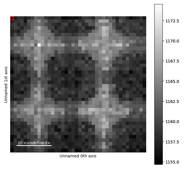
Removing dead pixels

Most detectors will have some dead pixels, with zero counts. There are several ways to locate them. The easiest being summing all the probe positions and then seeing which pixels have zero counts. Alternatively, an image with a flat illumination can be acquired on the detectors, and the dead pixels can be found from this.

The dataset from dummy_data has no “dead pixels”, so this processing won’t do much. The dataset from Zenodo has several dead pixels.

Use the function find_dead_pixels():

>>> s_dif = s.mean(axis=(0, 1))
>>> s_dead_pixels = s_dif.find_dead_pixels(lazy_result=False, show_progressbar=False)
>>> s_dead_pixels.plot()

For some datasets, like the one from Zenodo, s_dead_pixels will also show dead pixels at the corners of the detectors. This is due to no electrons hitting the detectors at these high scattering angles, caused by the pole piece of microscope blocking these. However, since this region is (typically) not very interesting, it does not matter that the algorithm incorrectly thinks these positions are dead pixels.

To correct for these dead pixels, use correct_bad_pixels(). This function can also be used to correct for hot pixels, using find_hot_pixels().

>>> s = s.correct_bad_pixels(s_dead_pixels)

By default this returns a lazy signal, which can be used in further processing. If for some reason processing this new signal is really slow and too big to process in memory, one trick can be to save it first with with an appropriate chunking (s.save("data_saved.hpsy, chunks=(32, 32, 32, 32))), then load it again (s = hs.load("data_saved.hspy", lazy=True)).

Finding the centre position

To do radial average of the datasets, we first need to find the centre position of the diffraction patterns. The easiest way of doing this is using center_of_mass()

>>> s_com = s.center_of_mass(threshold=2, show_progressbar=False)
>>> s_com
<DPCSignal2D, title: , dimensions: (2|40, 40)>
>>> s_com.plot()

This returns a DPCSignal2D object, which is another specialized class for analysing disk shifts (for example from magnetic materials). For more information about how to use this for analysing magnetic materials see the Jupyter notebook link from Ferromagnetic STEM-DPC analysis.

The first navigation index is the beam shifts in the x-direction, and the second is the beam shifts in the y-direction.

Doing the radial average

The next step is radially averaging the dataset as a function of distance from the centre position, which is done using radial_average().

>>> s_radial = s.radial_average(centre_x=s_com.inav[0].data, centre_y=s_com.inav[1].data, show_progressbar=False)
>>> s_radial
<Signal1D, title: , dimensions: (40, 40|62)>
>>> s_radial.plot()

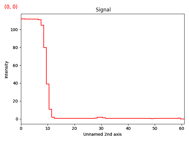
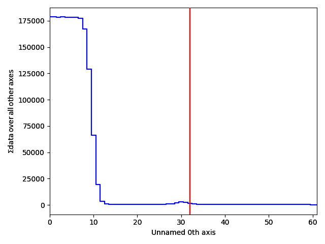
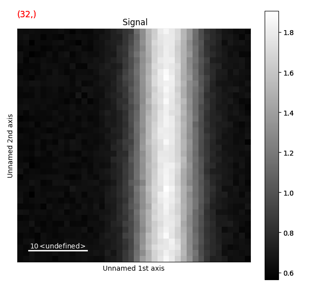
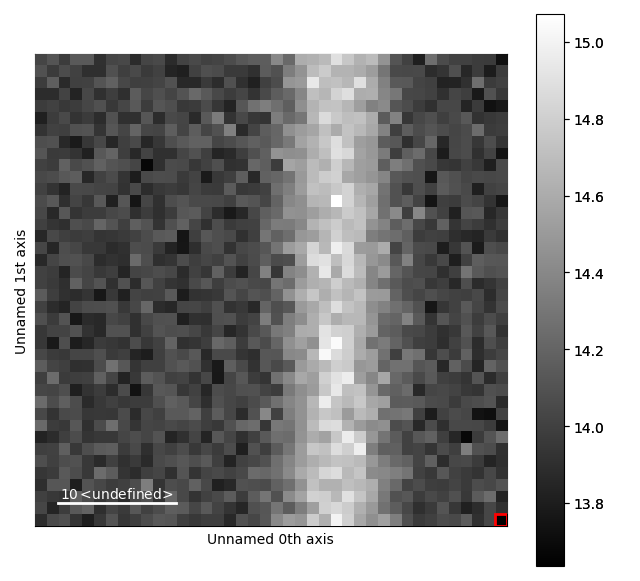
Now, the ring seen earlier is visible as a peak at x=30 in the signal plot.

A nice way of visualizing this is by transposing the signal, which swaps the signal and navigation axes. Plot the signal, and move the red line in the navigator plot to x=32.

>>> s_radial.T.plot()

Modelling the HOLZ ring

Having reduced the dataset from 4 to 3 dimensions, the HOLZ ring (now a peak, due to the radial average) can easily be fitting with a Gaussian function.

Firstly we extract parts of the signal related to the peak, and create a model.

>>> s_radial_cropped = s_radial.isig[20:40]
>>> m_r = s_radial_cropped.create_model()

Due to the noise, the mean value outside the peak is not zero. To account for this, we fit an offset component to the parts of the signal not containing the peak. For real datasets, a PowerLaw component should be used (instead of the Offset component).

>>> from hyperspy.components1d import Offset
>>> offset = Offset()
>>> m_r.set_signal_range(20., 25.)
>>> m_r.set_signal_range(37., 40.)
>>> m_r.append(offset)
>>> m_r.multifit(show_progressbar=False)
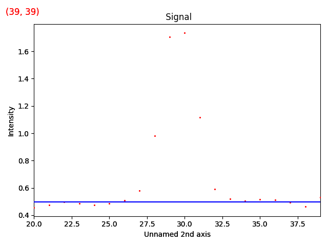
>>> m_r.reset_signal_range()
>>> m_r.plot()

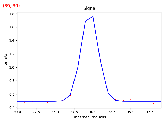
Then add a Gaussian function to this model.

>>> from hyperspy.components1d import Gaussian
>>> g = Gaussian(A=10, centre=30, sigma=4)
>>> m_r.append(g)
>>> g.centre.bmin, g.centre.bmax = 25, 35
>>> m_r.multifit(fitter='mpfit', bounded=True, show_progressbar=False)
>>> m_r.plot()

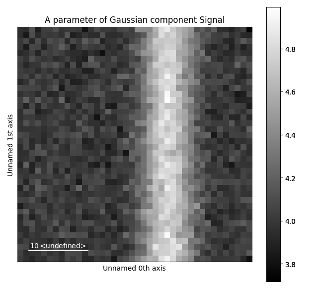
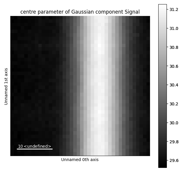
The various parameters in the Gaussian can then be visualized.

>>> g.A.plot()
>>> g.centre.plot()