Analysing NBED data

The analysis of this type of data in pixStem is based upon finding the position of diffraction disks, and using that for further analysis. This includes various pre-processing functions, for template matching the images with a binary disk and remove the background in the diffraction patterns. Lastly, the intensity from all the diffraction spots can be extracted.

It does not assume there are a limited number of structures or orientations within the dataset. All functions can be run “lazyily”, meaning all the data does not have to be loaded into memory. This make is possible to process data which is much larger than the available computer memory. Secondly, all the functions can be run in a parallel fashion over several cores. So more CPUs: faster processing.

For more extensive analysis of this type of data, especially acquired using precession, see pyXem: https://pyxem.github.io/pyxem-website/, which has more functions for extracting information about the crystal structure.

Imports and data

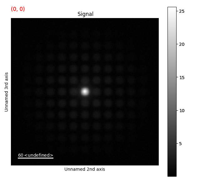
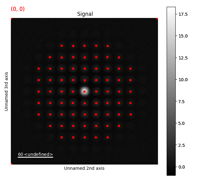
The signal we’re going to look at resembles a nanobeam electron diffraction pattern, acquired with a fast pixelated direct electron detector in scanning transmission electron microscopy mode. The convergence angle of the beam is sufficiently low, to avoid overlap between the diffraction disks.

Within the datasets, the crystal structure is the same, but contains some grains which are rotated along the axis parallel to the electron beam.

>>> import pixstem.api as ps
>>> s = ps.dummy_data.get_nanobeam_electron_diffraction_signal()
>>> s.plot()

Finding the peaks

The simplest way to locate the diffraction disks is to run a peak finding algorithm, without running any pre-processing, using the find_peaks() function in the PixelatedSTEM class.

This method can be run with difference of Gaussians (DoG) or Laplacian of Gaussian (LoG) peak finding routines, and has many parameters which can (and most often should) be tuned for your specific datasets. For a full list of these parameters, see the docstring (find_peaks()). For more information about how the parameters affect the peak finding, see skimage’s Difference of Gaussian and Laplacian of Gaussian docstrings.

>>> peak_array = s.find_peaks(lazy_result=False, show_progressbar=False)

This returns a NumPy array (or dask array if lazy_result=True) with the probe position in the first two dimensions. To access the peaks positions for a specific probe position, the peak_array can be sliced.

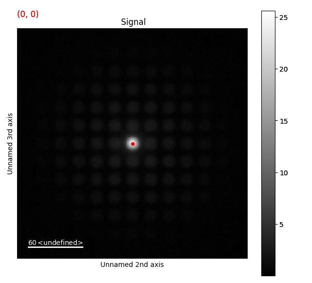
>>> peak_array[5, 2] 

It has only found one peak, the centre disk, since it is the most intense feature in the diffraction images! This is common in datasets such as these. It is possible to tune the peak finding parameters to find more of the disks, however this is often a tedious process. Especially for more tricky datasets, with for example randomly oriented diffraction patterns, where the intensity and disk shapes can vary a great deal.

(If you want to try to find more peaks in the dataset by tuning the parameters, the threshold is a good place to start. For example by starting with a value of threshold=0.05. However, in more complicated datasets this can also lead to an increase in false positives.)

Another way of finding the disks is doing some pre-processing of the diffraction images, by utilizing the shape of the diffraction disks.

Template matching with peak finding

One advantage with acquiring the data with a convergent beam, is that the diffraction spots become disks. These disks are easy to separate from the wide range of others features in the diffraction images, like cosmic rays or other types of noise.

A fairly easy way of finding these disks is by cross-correlating each diffraction image with a binary disk: template_match_disk(). The only input parameter is the radius of this disk, disk_r. For this dataset, lets set disk_r=5.

>>> st = s.template_match_disk(disk_r=5, lazy_result=False, show_progressbar=False)
>>> st.plot()

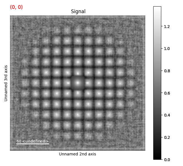
This returns a new dataset, with the same size as the original dataset. Here, the disks are much more visible, and we can apply the peak finding directly on this template matched dataset.

>>> peak_array = st.find_peaks(lazy_result=False, show_progressbar=False)

To visualize them on the template matched signal, we use add_peak_array_as_markers(). This peak_array can also be added to the original signal, to see how well the peak finding worked. To delete the markers, run: del s.metadata.Markers

>>> st.add_peak_array_as_markers(peak_array)
>>> st.plot()
>>> s.add_peak_array_as_markers(peak_array)
>>> s.plot()

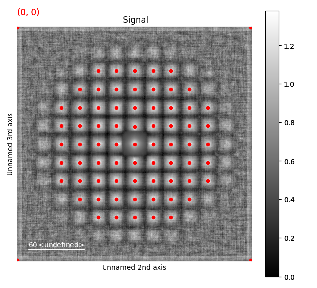
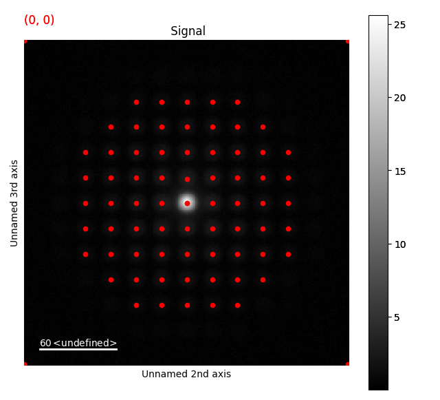
This seems to have worked pretty well!

Refining peak positions

Next, we can refine each peak position using centre of mass, using peak_position_refinement_com():

>>> peak_array_com = s.peak_position_refinement_com(peak_array, lazy_result=False, show_progressbar=False)

We compare before and after by using a different color for the peak_array_com.

>>> s.add_peak_array_as_markers(peak_array_com, color='blue')
>>> s.plot()

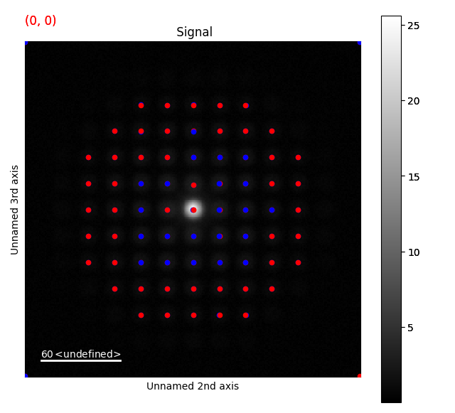
This had some effect, but especially towards the very intense centre part of the diffraction image, the peaks are obviously shifted due to the background.

Removing background

The background is removed with subtract_diffraction_background(). There are several ways for removing the background, with a range of parameters: difference of gaussians, median kernel and radial median. Lets go with the default: median kernel.

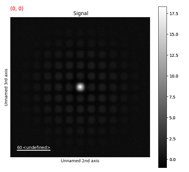
>>> s_rem = s.subtract_diffraction_background(lazy_result=False, show_progressbar=False)
>>> s_rem.plot()

Then we can apply the same center of mass refinement, using the peak_array we already calculated.

>>> peak_array_rem_com = s_rem.peak_position_refinement_com(peak_array, lazy_result=False, show_progressbar=False)
>>> s_rem.add_peak_array_as_markers(peak_array_rem_com)
>>> s_rem.plot()

Extracting disk intensity

Lastly, we can extract the intensity from each of the diffraction spots using intensity_peaks():

>>> peak_array_intensity_rem = s_rem.intensity_peaks(peak_array_rem_com, lazy_result=False, show_progressbar=False)

This returns a NumPy array similar to the one we’ve seen earlier, but with an extra column. To extract a single peak from a single position:

>>> peak_array_intensity_rem[5, 2][10]